ctl.ControlSBML

controlSBML provides ways to use an SBML model to construct an object representing a system model that can be used by the control package. Two kinds of control objects can be constructed. The first, control.NonlinearIOSystem, wraps an entire nonlinear SBML model. This allows the control package to do the same kind of detailed simulations that are provided by SBML simulators as as libroadrunner and Copasi. The second object, control.StateSpace, provides a linear approximation to the SBML model. control.NonlinearIOSystem and control.StateSpace objects are constructed from an ctl.ControlSBML object.

In the sequel, we use the following Antiimony representation of an SBML model.

SIMPLE_MODEL = """
    species E1;
    J1: S1 -> S2; S1 + E1
    S1 = 10; S2 = 0; E1 = 1;
"""

Constructors

We begin with constructing a ctl.ControlSBML object. This requires having a representation of an SBML model. This can be an XML file, an XML URL, an antimony file, or a libroadrunner object. We refer to any of these representations of the SBML model as a model reference. The following constructs ctl.ControlSBML object for this model.

ctlsb = ctl.ControlSBML(SIMPLE_MODEL)

This object has a number of useful properties.

• ctlsb.antimony is the Antimony string that corresponds to the model reference in the constructor.

• ctlsb.roadrunner is the libroadrunner object for the model reference in the constructor.

• ctlsb.state_ser is a pandas Series that provides the values of the concentrations of floating species (the state variables).

• ctlsb.setTime(time) runs the simulation from time 0 to a desired time. This updates ctlsb.state_ser.

To create an object that is more useful for control analysis, you should specify at least one input and at least one output. An input is a chemical species that can be manipulated by increasing or decreasing its value. An output is a chemical species or reaction flux that can be read. An example of this constructor is:

ctlsb = ctl.ControlSBML(SIMPLE_MODEL,
    input_names=["E1"], output_names=["S2"])

Note that both input_names and output_names are lists of strings. Inputs and outputs must be specified to make use of subsequent capabilities of ctl.ControlSBML.

control.NonlinearIOSystem

The method ctl.ControlSBML.makeNonlinearIOSystem constructs a control.NonlinearIOSystem object for an SBML model. The control.NonlinearIOSystem object provides a way to use many of the capabilities of the control system library. For example,

ctlsb = ctl.ControlSBML(SIMPLE_MODEL,
        input_names=["E1"], output_names=["S1", "S2"])
sys = ctlsb.makeNonlinearIOSystem("simple")

sys is a control.NonlinearIOSystem object, and the following simulates this system for 5 s.

times = [0.1*n for n in range(51)]
time_response = control.input_output_response(sys,
    times, X0=ctl.makeStateVector(sys))

ctlsb is constructed to have the input E1 and the outputs S1 and S2. sys is a control.NonlinearIOSystem object that wraps the SBML model. time_response is a control.TimeResponseData object. The simulation requires knowlege of initial values for all state variables, which is provided by the method ctl.makeStateVector.

Going a bit further, we introduce a plotting function for the control.TimeResponseData object.

def plotTimeResponse(time_response, output_names,
      is_legend=True, stmts=None):
    # Plots the results of running a simulation
    outputs = time_response.outputs
    times = time_response.time
    colors = ["orange", "green"]
    for idx in range(len(output_names)):
        if np.ndim(outputs) > 1:
            plt.plot(times, outputs[idx,:], c=colors[idx])
        else:
            plt.plot(times, outputs, c=colors[idx])
    if is_legend:
        _ = plt.legend(output_names)
    if stmts is None:
        stmts = []
    for stmt in stmts:
        exec(stmt)
    plt.xlabel("time")
    plt.ylabel("concentration")

We execute the statement below to plot the simulation results.

plotTimeResponse(time_response, ["S1", "S2"])

control.StateSpace

A state space model is a linear system of differential equations in which there are \(n\) states, \(p\) inputs, and \(q\) outputs.

\[\begin{split}\dot{\bf x} &= {\bf A} {\bf x} + {\bf B} {\bf u} \\ {\bf y} &= {\bf C} {\bf x}\end{split}\]

where:

\[\begin{split}{\bf x} \text{ has dimension } n \times 1 \\ {\bf u} \text{ has dimension } p \times 1 \\ {\bf y} \text{ has dimension } q \times 1 \\ {\bf A} \text{ has dimension } n \times n \\ {\bf B} \text{ has dimension } n \times p \\ {\bf C} \text{ has dimension } q \times p \\\end{split}\]

\({\bf x}\) is the state variable, \({\bf u}\) is the input vector, and \({\bf y}\) is the output.

controlSBML constructs a control.StateSpace object for an SBML model as follows. The state variables are floating species. The \({\bf u}\) are names of floating species that are manipulated inputs (input_names). The \({\bf y}\) are the names of measured outputs (output_names), either floating species or names of reactions whose fluxes are output. A linear approximation for an SBML model is constructed using the Jacobian of the state variables at a specified operating point. The operating point is a simulation time at which state variables are assigned their values to calculate the Jacobian.

Once a ctl.ControlSBML object has been constructed, the method makeStateSpace is used to create a control.StateSpace object. This is illustrated below to construct a control.StateSpace object using time 0 as the operating point.

ctlsb = ctl.ControlSBML(SIMPLE_MODEL,
    input_names=["S1"], output_names=["S2"])
state_space = ctlsb.makeStateSpace(time=0)

The resulting state space model is represented below. \({\bf x}\) is a 3 dimensional vector that correspond to the state variables (floating species) E1, S1, and S2. \(u\) and \(y\) are scalars (and so are not in bold). \({\bf A}\) is in the upper left; \({\bf B}\) is in the upper right; and \({\bf C}\) is in the lower left. \({\bf A}\) is A \(3 \times 3\) matrix; \({\bf B}\) is a \(3 \times 1\) matrix; and \({\bf C}\) is \(1 \times 3\).

We can construct a transfer function from a control.StateSpace object. The transfer function for the above system is obtained by

transfer_function = control.tf(state_space)

and is displayed as

The DC gain for this transfer function is \(\infty\). This makes sense since by having a unti input for times \(\geq 0\) and a single reaction that consumes S1 to produce S2, the output increases without bound.

Now consider a slightly different reaction network.

model = """
    J1: S1 -> S2; S1
    J2: S2 -> S1; S2
    J3: S2 -> ; k*S2
    S1 = 10; S2 = 0;
    k = 0.8
"""

ctlsb = ctl.ControlSBML(model,
      input_names=["S1"], output_names=["S2"])
state_space = ctlsb.makeStateSpace()

The state space matrices are:

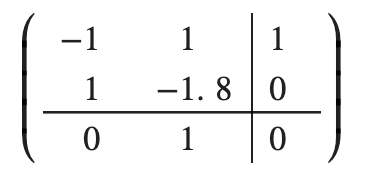
We simulate and plot the response of the state space model to a unit step in the input in S1.

times = [0.1*n for n in range(301)]
ss_time_response = control.forced_response(state_space,
      times, X0=[10, 0], U=1)
plotTimeResponse(ss_time_response, ["S2"], is_legend=False)
plt.plot([0, 30], [1.25, 1.25], linestyle="--")

The transfer function is

and so the DC gain is \(1/0.8=1.25\), which is consistent with the plot.