System Identification
controlSBML methods that can assist with fitting a SISO transfer function
to an SBML model.
There is one preparatory step and then
two analysis steps.
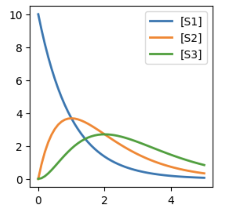
To illustrate these steps, we introduce the following LINEAR_MODEL:
 1LINEAR_MODEL = """
 2J1: S1 -> S2; k1*S1
 3J2: S2 -> S3; k2*S2
 4J3: S3 -> ; k3*S3
 5S1 = 10; S2 = 0; S3 = 0
 6
 7k1 = 1
 8k2 = 1
 9k3 = 1
10"""
Simulating this model produces the output below:
In the preparatory step, we construct a SISOTransferFunctionBuilderObject.
This involves first constructing a ControlSBML object and from this
obtaining a SISOTransferFunctionBuilder object.
For the former, we specify S1 as the input to the system,
and S2 as the output.
linear_ctlsb = ctl.ControlSBML(LINEAR_MODEL,
      input_names=["S1"], output_names=["S3"])
linear_builder = linear_ctlsb.makeSISOTransferFunctionBuilder()
The constructor for SISOTransferFunctionBuilder has a number of optional keyword
arguments, such as specifying as providing a way to explicitly specify the
input and output names of the SISO system.
Now we are ready for the first analysis step–evaluating the operating region for the SISO system.
This is done by examining the relationship between values of the input, S1 in our
example, and the output, S3.
This relationship is assessed by presenting the SISO system with a staircase of
input values.
A staircase is a sequence of step inputs that have the same change in magnitude and time duration.
linear_builder.plotStaircaseResponse(initial_value=2, final_value=10, num_step=5,
      figsize=(3,3), legend_crd=(0.5, 1), end_time=100)
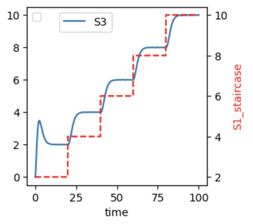
The staircase is specified by initial_value, final_value, and num_step.
Various plotting options are available as well.
The left y-axis of the plot is for the output (S3), and the right y-axis is for the staircase function.
We see that the output changes in close connection with changes in the input.
Sometimes you will need to lengthen the simulation time in order for the system
to settle to see these changes.
In the second analysis step, we determine an appropriate transfer function for the SBML model. The approach here is to find a transfer function that accurately predicts the system output from its input over the operating region. The workflow is:
The user chooses a degree of the numerator and denominator polynomials of the transfer function.
The user runs the method
fitTransferFunction.If the fit is good, the user may consider reducing the degree of the numerator and/or denominator polynomials to avoid overfitting.
If the fit is poor, the user may increase the degree of the numerator and/or denominator polynomials.
If the fit is good and the polynomials have a low degree, this step is completed.
fitter_result = linear_builder.fitTransferFunction(
      1, 2, final_value=10, initial_value=2, end_time=100)
ctl.plotOneTS(fitter_result.time_series,
      figsize=(3,3), legend_crd=(2,1))
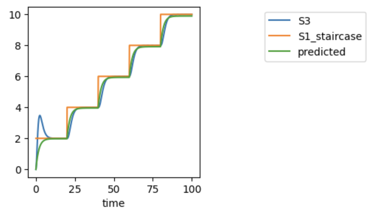
We see that the predicted value of S3 coincides closely with the value of S3 from
the nonlinear simulation.
So, it seems that we have a good transfer function.
The control.TransferFunction object is in fitter_result.transfer_function;
it is \(\frac{5.368}{10s + 5.424}\).
Other useful properties are:
nfevis the number of different transfer functions that were evaluated to find the fitparameterscontains the parameter valuesredchiis the reduced ChiSq for the fitstderrcontains the standard deviations of the parameter valuestime_seriesis aTimeseriesobject with the input, nonlinear simulated output, and predicted value of the outputtransfer_functionis the fitted transfer function.